The Problem with Explaining Black Boxes
Imagine a bank deploys a machine learning model to decide loan applications. A customer is denied credit and they ask for an explanation. The bank runs LIME, a popular explanation method, and learns that "employment length" was the most important factor. Reassured, they share this with the customer. But had they run LIME again, they might have gotten a different answer: "account balance" was most important. A third run might point to "age." Same model, same applicant, three different stories.
This isn't a contrived scenario. It's a well-documented weakness of perturbation-based explanation methods. The approaches like LIME, GLIME, BayesLIME, and others work by generating random perturbations around an input, querying the black-box model, and fitting a simple surrogate to approximate local behavior. The idea is elegant, but the execution has a fundamental flaw: the quality of the explanation depends entirely on which perturbations you happen to sample.
Random or heuristic sampling leads to explanations that vary across runs, miss important regions of the input space, and provide no measure of how confident we should be in the result. When explanations are unstable and come without uncertainty estimates, they can be worse than no explanation at all, they create a false sense of understanding.
This raises a natural question:
If we only get a limited budget of black-box queries, how should we choose perturbations to learn the most about what the model is doing locally, and how confident can we be in the resulting explanation?
This is the question our work, EAGLE (Expected Active Gain for Local Explanations), sets out to answer. Rather than treating perturbation generation as a preprocessing step, EAGLE reframes it as a sequential decision problem: at each step, choose the perturbation that will teach us the most about the model's local behavior.
Why Existing Methods Fall Short
To understand what EAGLE does differently, it helps to see where current methods struggle. The figure below (from our paper) shows how different methods sample perturbations around a target instance on a simple 2D dataset.
LIME and BayLIME sample broadly in the vicinity of the instance but ignore regions where the surrogate model is uncertain. They may waste queries on areas that are already well-understood. GLIME goes to the other extreme — constraining perturbations so tightly around the instance that it misses the broader local structure, including the decision boundary. BayesLIME does consider uncertainty, but only through predictive variance, which doesn't account for the locality of new candidates. It can drift toward uninformative regions far from the instance.
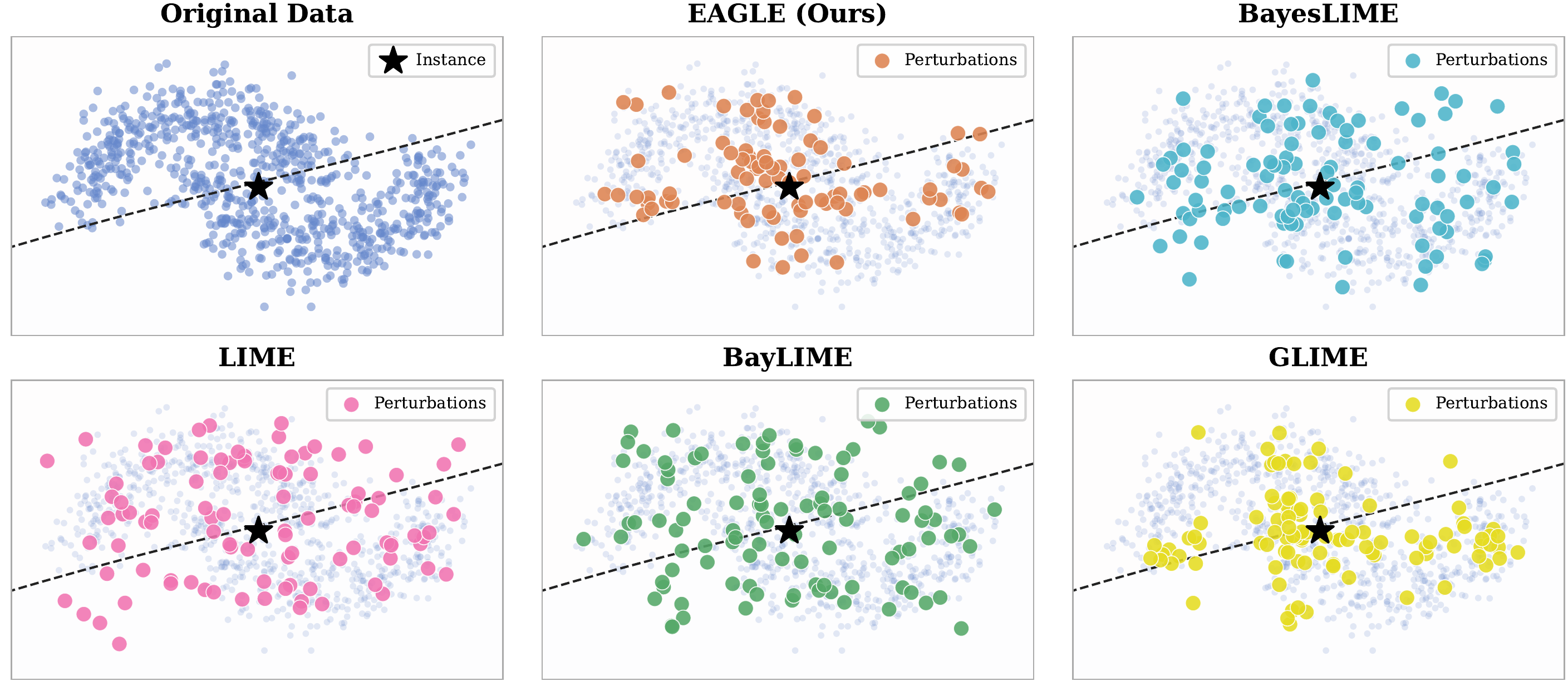
The common thread? None of these methods jointly optimize for where uncertainty is highest and where locality matters most. They either ignore uncertainty, ignore locality, or treat them separately. EAGLE is designed to handle both simultaneously.
EAGLE: Active Learning Meets Explainability
EAGLE reframes perturbation selection for post-hoc explanations as an information-theoretic active learning problem. The core idea is simple: instead of generating perturbations blindly and hoping they're informative, EAGLE iteratively asks — "given everything I've learned so far, which perturbation would teach me the most about the model's local behavior?"
The framework builds on a Bayesian linear regression (BLR) surrogate, which naturally provides uncertainty estimates over feature attributions through posterior distributions. EAGLE replaces heuristic perturbation selection with a principled acquisition function derived from expected information gain (EIG).
Here's how a single explanation is produced:
The Acquisition Function: Where the Magic Happens
The key theoretical result of our work (Theorem 1) shows that maximizing the expected information gain in the Bayesian linear surrogate simplifies to an elegant closed-form acquisition rule:
This expression is deceptively simple, but packs two crucial ideas into a single product:
The uncertainty term $\mathbf{z}^\top V_\phi \mathbf{z}$ measures how much the candidate perturbation $\mathbf{z}$ aligns with directions in feature space where the surrogate model's parameters are still uncertain. Think of the posterior covariance $V_\phi$ as an ellipsoid representing "what we don't know yet" — this term picks perturbations that probe the longest axes of that ellipsoid, where a new observation would collapse the most uncertainty.
The locality kernel $\pi_{x_0}(\mathbf{z})$ ensures that we don't chase uncertainty into irrelevant regions of the input space. An informative perturbation on the far side of the dataset might reduce posterior variance, but it tells us nothing about what the model is doing near our instance of interest. The locality weight keeps sampling focused.
The product of these two terms is what makes EAGLE unique. Existing methods handle them separately or ignore one entirely. BayesLIME, for instance, evaluates $\mathbf{z}^\top V_\phi \mathbf{z}$ (scaled by a global factor $s^2$) but does not incorporate the locality kernel when selecting new candidates — it only uses locality when fitting the surrogate to already-observed points. This subtle but important gap means BayesLIME's sampling can drift away from the neighborhood that matters.
Theoretical Guarantees
A key advantage of EAGLE's principled derivation is that it enables formal theoretical analysis — something rarely available for perturbation-based explainers. Most existing methods are designed by intuition and validated only empirically. EAGLE comes with provable bounds that tell us exactly what to expect.
The Diminishing Returns Phenomenon
We prove (Lemma 1) that the cumulative information gained under EAGLE's acquisition strategy grows as $\mathcal{O}(d \log t)$, where $d$ is the feature dimension and $t$ is the number of queries. What does this mean practically?
The first few perturbations are enormously informative, they rapidly carve out the shape of the local decision boundary. But each subsequent perturbation teaches a little less than the one before. This is good news, as it means EAGLE front-loads the most valuable queries. If the query budget is tight, EAGLE extracts maximum value from every single black-box call. The multiplicative factor $d$ tells us that higher-dimensional problems need proportionally more queries, which matches intuition as more features means more directions to explore.
How Many Queries Do We Need?
We derive high-probability bounds on the estimation error of the explanation weights (Theorem 2), which lead to a concrete sample complexity result:
This shows that we'll need quadratically more queries for tighter explanations, that's the price of precision. But for higher confidence (smaller $\delta$, i.e., stronger guarantees that the explanation is close to the truth)? That only costs a mild logarithmic penalty. In a credit scoring model with 20 features, for instance, we can get a reliable explanation with a budget that scales as roughly $20 \times \log(\text{confidence})$, not $20^2$, and EAGLE tells us exactly when to stop querying.
Does It Actually Work? Empirical Results
We evaluated EAGLE across six datasets: four tabular (COMPAS, German Credit, Adult Income, Magic Gamma Telescope) and two image (MNIST, ImageNet); against eight baselines including LIME, GLIME, BayLIME, BayesLIME, US-LIME, Tilia, DLIME, and UnRAvEL. The short answer: EAGLE consistently outperforms across the board.
Explanation Stability
We measured the pairwise Jaccard similarity of top-5 features across repeated explanation runs. EAGLE consistently achieves the highest or near-highest stability across datasets. Notably, while some baselines like Tilia or GLIME shine on individual datasets (Tilia on COMPAS, GLIME on ImageNet), their performance varies considerably across tasks. EAGLE is the only method that maintains consistently strong performance across both tabular and image domains.
| Method | COMPAS | German | Adult | MAGIC | MNIST | ImageNet |
|---|---|---|---|---|---|---|
| LIME | 0.772 | 0.645 | 0.669 | 0.647 | 0.733 | 0.704 |
| GLIME | 0.635 | 0.546 | 0.559 | 0.624 | 0.519 | 0.920 |
| Tilia | 0.834 | 0.721 | 0.783 | 0.647 | 0.733 | 0.734 |
| BayesLIME | 0.770 | 0.631 | 0.674 | 0.617 | 0.765 | 0.755 |
| BayLIME | 0.779 | 0.678 | 0.663 | 0.648 | 0.720 | 0.739 |
| EAGLE (Ours) | 0.802 | 0.775 | 0.822 | 0.785 | 0.861 | 0.825 |
Sampling Quality & Convergence
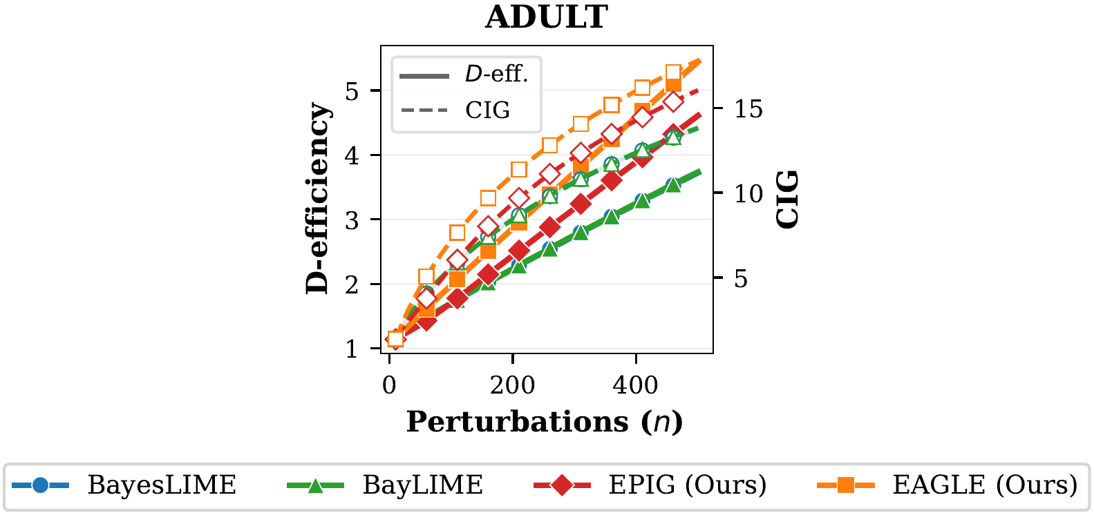
We measured D-efficiency (reduction in posterior covariance volume) and cumulative information gain (CIG) as perturbations are acquired. EAGLE exhibits a steeper convergence trajectory from the very first acquisition steps. At n=500, it achieves roughly 1.5× the D-efficiency of BayesLIME and BayLIME. More importantly, the D-efficiency curves grow linearly in the plot (logarithmically in $t$), exactly matching the $\mathcal{O}(d \log t)$ scaling predicted by our Lemma 1. It's reassuring when theory and experiments agree.
Sample Efficiency: Doing More with Less
We measured how many queries EAGLE needs to match the performance that BayesLIME achieves at its full budget of 500 queries. On D-efficiency, EAGLE matches BayesLIME@500 using only 310–390 queries, a saving of 22–38%. On the CCM metric (which combines sign stability and rank consistency), the savings are even more dramatic: 52–88%. On MNIST, EAGLE at just 60 queries produces explanations as consistent as BayesLIME at 500.
And It's Faster Too
One might expect the active learning loop to add computational overhead, but EAGLE is actually faster than BayesLIME. At N=500 on COMPAS, EAGLE takes 8.16 seconds versus BayesLIME's 14.56 seconds — a nearly 44% reduction. The reason? EAGLE's acquisition function has a closed-form solution (a matrix-vector product), avoiding the expensive optimization loops that other Bayesian methods require. On ImageNet, the speedup is even more pronounced: 7.08s versus 34.73s.
Tighter Uncertainty: Knowing What We Don't Know
Beyond producing stable point estimates, EAGLE yields significantly narrower credible intervals on feature attributions. The 90% posterior credible intervals from EAGLE are consistently tighter than those from BayesLIME and BayLIME across all features, meaning practitioners can more confidently separate genuinely important features from noise.
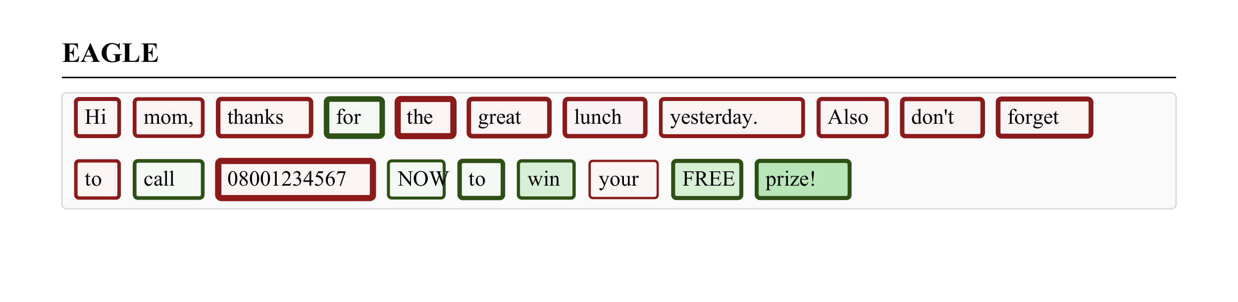
To make this concrete, consider a spam detection example from our paper. Given the message "Hi mom, thanks for the great lunch yesterday. Also don't forget to call 08001234567 NOW to win your FREE prize!", EAGLE's explanation correctly highlights spam-indicative words like "FREE," "prize," "NOW," and "win" with strong positive attributions (green), while personal words like "mom," "thanks," and "lunch" get negative attributions (red, i.e., evidence against spam). Crucially, the border thickness around each word encodes the uncertainty — and EAGLE's borders are thin, meaning it's confident in these attributions.
The Bigger Picture
Post-hoc explanation methods sit at a critical juncture in the AI pipeline. They're often the last line of defense between an opaque model and the people affected by its decisions. If these explanations are unreliable, the entire accountability chain breaks down.
EAGLE addresses this at a foundational level. By recasting perturbation selection as an information-theoretic optimization problem, it shifts the paradigm from "generate perturbations and hope for the best" to "systematically extract the maximum amount of local information from every black-box query." The result isn't just better numbers on a benchmark, it's explanations that practitioners can actually trust, backed by both theoretical guarantees and empirical evidence.
Principled acquisition: EAGLE derives a closed-form acquisition function from information-theoretic first principles, replacing ad-hoc heuristics with a mathematically grounded strategy.
Theoretical guarantees: $\mathcal{O}(d \log t)$ information gain bounds and sample complexity guarantees, rare in the post-hoc explainability literature, and practically useful for budgeting queries.
Consistent improvements: Higher stability, faster convergence, tighter uncertainty, and lower runtime across both tabular and image benchmarks.
Looking Ahead
EAGLE opens several exciting research directions. The current greedy top-B batch selection could be replaced with batch optimal strategies that account for redundancy between selected perturbations. Extending the framework to non-linear surrogates, perhaps using Bayesian neural networks or Gaussian processes could capture more complex local decision boundaries.
More broadly, we see EAGLE as evidence that the tools of Bayesian experimental design and active learning, have a natural and important role to play in making AI systems more transparent. The explanations we produce should be held to the same standards of rigor as the models they explain.
Read the full paper